Graph IDE ► Data Graphics ► Scatter
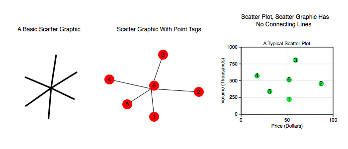
A scatter is a sequence of points. Those points may be connected to a common point, usually the mean of the points. A scatter is very similar to a Polygon (see Polygon) except for the way that the points are connected. The figures below show examples of the use of scatters.
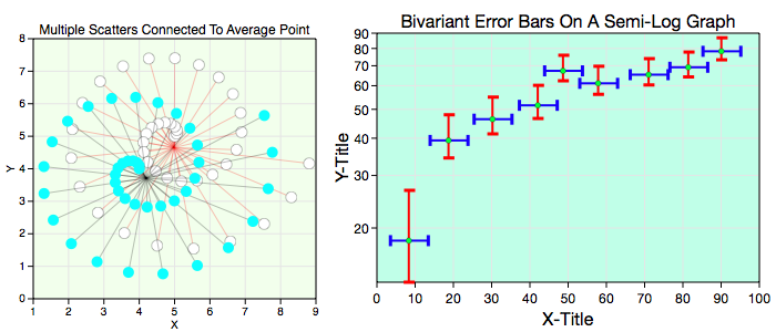
Scatter graphics support the concept of a Network, are simply an element of a Layer in either an overlay or graph and transform according to the properties of a coordinate per the Non-Linear Graphs rules. As such, scatter graph and indeed any data graphic support attributes that can make them far superior to a simple scatter graphic canonical form. The figure below shows some examples of that.
Some standard operations are itemized below.
Data Editor
The Data Editor for the Scatter Graphic is shown below.
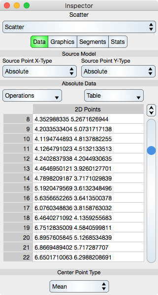
Source Model
A description of the Source Model is the same as for the Function graphic.
Note that for the Bivariant Error Bar graph shown above there are six scatter graphics. Two represent the data and the other four represent the error data. The four have their Source Model set to be relative to the two data scatter graphics. It is a bit tedious to setup and modify as the data is contained in the representation, however if the data resides in a Spreadsheet then data adjustments become much more direct.
Table
Operations : Select this to perform common sequence operations upon the data. The most important sequence operation is Switch X and Y because that transposes the data and hence the dimensions. Contrast this to the Function graphic which assumes that x is alway ascending and always the independent variable of the coordinate system (graph).
Generic table controls are described in the Tables section.
The rows represent vertex values. While in Atomic mode, the cell represents a point (x and y value) and while in component mode the cell represents either a x or y value. Hence, in atomic mode there is one column while in component mode there are two columns.
Center Point Type
Center Point Type : Scatter graphs are typically unconnected representations. However, data can be connected in sequence order, to the average point, median point or to the zero point (None, Average, Median and Zero). If connected in sequence order then the scatter graph is often referred to as a trajectory graph. Since trajectories are often smooth that designation is reserved for the Trajectory graphic which is points connected by Cubic Bezier spline sections.
If None then the data points are connected in sequence by line segments. Turning off the stroke in the graphic editor turns off the connected segments and results in a classic scatter representation.
Graphics Editor
The Graphics Editor for the Scatter graphic is shown below.
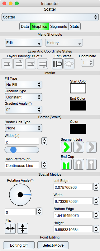
Common Controls
Controls common to all graphics are described in the Graphics section.
Coordinate : When the scatter resides on a Multiple Coordinate Graph then the coordinate control is used to define which coordinate it resides on.
Point Editing
Editing Off/On : Places the graphic into or out of edit mode. While in edit mode the vertices are shown by indicators and can be adjusted using mouse or touch events. Double-clicking the graphic also toggles this edit mode.
Select/Move or Add/Delete : Select/Move mode permits the vertex editing to select and move those locations while Add/Delete mode will delete a vertex if it is hit or add a vertex if a Scatter segment is hit. This can also be accomplished using the shift key if available.
Segments Editor
The Segments Editor for the Scatter graphic is shown below.
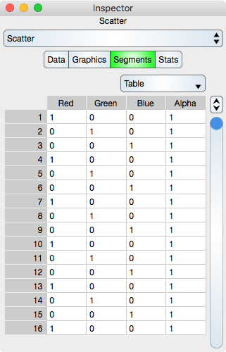
Segments are the line segments between adjacent points. See Sequence Colors for additional information.
Table
Table controls are described in the Tables section.
The rows represent a segment color values. While in Atomic mode, the cell represents a rgba value and while in component mode the cell represents either single r, g, b and a. Hence, in atomic mode there is one column while in component mode there are four columns.
Note that if the Data sequence is resorted then the Segments sequence will not be resorted.
Stats Editor
The Stats Editor shows basic statistics for the Scatter graphic and is shown below.
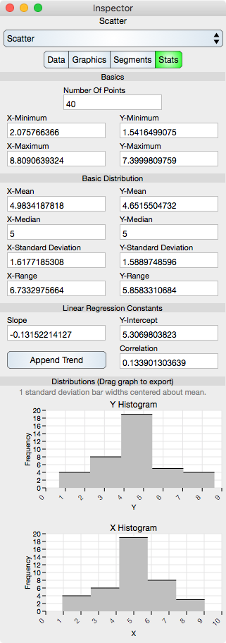
Basics
Number Of Points : Shows the number of points in the Scatter.
X-Minimum : x-minimum value of all the data points.
Y-Minimum : y-minimum value of all the data points.
X-Maximum : x-maximum value of all the data points.
Y-Maximum : y-maximum value of all the data points.
Basic Distribution
The basic distribution is shown separately for the x-dimension and the y-dimension.
Mean : Shows the mean of the data.
Median : Shows the median of the data.
Standard Deviation : Shows the standard deviation of the data.
Range : Shows the range of the data (maximum - minimum).
Linear Regression Constants
Note that linear regression may also be referred to as line fit.
Slope : Shows the slope of the linear regression.
Y-Intercept : Shows the y-intercept of the linear regression.
Correlation : Shows the correlation constant of the linear regression.
Append Trend : Places a new trend line over the scatter. The trend is a least squares fit and each data value of the scatter is also on the trend. Thus if the scatter is on a non-linear graph then the trend will map as well and not look like a linear fit on page view coordinates.
Distributions
Y Histogram : Shows the y-histogram of the data. This graph can be dragged onto the Graphic View.
X Histogram : Shows the x-histogram of the data. This graph can be dragged onto the Graphic View.